


Introduction
Air quality, predominantly affected by particulate matter (PM), is a critical determinant of public health and wellbeing. One of the most concerning pollutants in this category is PM2.5 atmospheric particulate matter with a diameter of less than 2.5 µ m. Owing to their minuscule size, these particles remain suspended in the air for prolonged periods, increasing the risk of inhalation and subsequent health complications. Notably, extended exposure to such particulate matter can lead to increased morbidity and mortality rates, predominantly due to cardiovascular diseases and respiratory symptoms [1].
Eastern Europe, especially countries such as Bosnia and Herzegovina (BiH), faces exacerbated challenges related to air pollution. Comparatively, regions within Eastern Europe experience more deleterious air quality than their Western counterparts do [2]. Ambient PM2.5 exposure levels in BiH often surpass the World Health Organization's (WHO) recommended threshold of 10 µ g/m3, making it a region with some of the most polluted air in Europe [3]. A 2019 report from Air Quality Management (AQM) in BiH indicated that air pollution results in 3,300 deaths annually in the country, with a staggering 81 % attributable to cardiovascular diseases [2]. The origins of this elevated PM2.5 concentration in BiH are multifaceted. Transport, coal-powered plants, industrial activities, agriculture, and the domestic burning of solid fuels are prime contributors. However, the extent of pollution varies geographically and is intricately linked to economic and social dynamics. Cities such as Sarajevo, Banja Luka, Lukavac, and Tuzla have alarmingly high pollution levels. Seasonal variations, particularly during winter, further accentuate the pollution problem, leading to episodes of dense smog and reduced visibility. Moreover, socio-economic disparities render certain demographics, notably the disadvantaged, more vulnerable due to their reliance on cheaper, more polluting fuels and outdated transportation [4]. Despite these alarming statistics, the monitoring infrastructure for PM levels in BiH remains underdeveloped, with many stations lacking the capacity to monitor PM2.5. Recognizing this data lapse, coupled with escalating pollution levels and the associated public health crisis, requires urgent intervention, and there is pressing need to develop innovative approaches for estimating the concentration levels.
Remote sensing offers a promising avenue in this direction. In recent decades, satellite-based instruments have revolutionized environmental monitoring capabilities [5]. Products from agencies such as National Aeronautics and Space Administration (NASA), National Oceanic and Atmospheric Administration (NOAA), and Copernicus have paved the way for in-depth aerosol studies, with Aerosol Optical Thickness (AOT) emerging as a vital air pollution indicator [6]. Notably, statistical models have been widely utilized to forecast the concentrations of air pollutants, which are vital for timely warnings and effective decision-making. Although effective, models such as dispersion and chemical transport models are computationally exhaustive and may not be cost-effective for routine predictions [7]. Consequently, the rise in machine learning (ML) and statistical models offers a promising solution to these challenges. Models, such as the Bayesian geostatistical model, Linear Regression (LR), and Random Forest (RF), have the advantage of discovering concealed data patterns without the need for deep knowledge of the physico-chemical characteristics of pollutants, thus enhancing the computational efficiency [1,8,9]. Such models are particularly crucial in light of increasing research that underscores the detrimental health effects of air pollution. For instance, Matkovic et al. [10] highlighted that PM2.5 pollution contributed substantially to adult mortalities in specific districts of BiH. Given the risks posed by particulate matter, especially PM2.5, which can induce cardiovascular diseases and respiratory infections, it is imperative to develop predictive models [11].
As the importance of ML and deep learning algorithms in atmospheric science grown, with a conspicuous concentration of studies in China, there is a concurrent trend to leverage satellite products for more accurate PM predictions [7,12,13]. While some studies suggest that meteorological parameters such as wind speed, solar radiation, precipitation, and relative humidity play a significant role in predicting PM2.5 concentration [14], others argue that they have minimal influence, highlighting the impact of other trace gases on distribution [15]. Interestingly, Hajiloo et al. [16] Incorporates derived indices along with meteorological parameters to estimate PM2.5 concentration and finds correlations in predicting concentration levels. Considering the evolving landscape of air pollution studies, this study bridges some gaps. such as leveraging remote sensing products, particularly United States Geological Survey (USGS) Landsat 8 Collection 2 Tier 1 and Real-Time data products and derived indices. By analyzing these variables in conjunction with ground truth PM2.5 datasets, this study seeks to explore the accuracy of these variables in influencing PM2.5 concentration prediction and examine how pollutant concentration levels vary with seasons. We hypothesize that the use of landsat 8 products and associated indices will be highly effective in predicting PM2.5 concentration levels, given their accessibility. This approach not only highlights the severity of the air pollution challenge in BiH but also offers a methodological blueprint that can be replicated in other regions facing similar issues.
Methods
Data acquisition and pre-processing
PM2.5 concentration data from January 2019 to December 2021 were sourced from OpenAQ database (available at https://explore.openaq.org/#12.96/44.53267/18.69241, accessed in July 2022) for five stations, named Zivinice, Lukavac, Bukinje, BKC, and Skver, all within Tuzla district. These data were obtained from reference-based sensor instruments operated by a government entity. The data, measured in µ g/m³, was downloaded in comma-separated value (CSV) format and subsequently cleaned using Microsoft Excel 2010. The dataset was divided into four seasons: December to February for Winter, March to May for Spring, June to August for Summer, and September to November for Autumn. Seasonal averages were calculated for the three-year period, and the concentration levels were ranked according to the United States Environmental Protection Agency (US EPA) standards (see Table 1).
Remote sensing data, specifically the USGS Landsat 8 Collection 2 Tier 1 and Real-Time Data Raw Scenes, were obtained using the Google Earth Engine (GEE) (available at https://developers.google.com/earth-engine/datasets/catalog, accessed in October, 2022). These data provide atmospheric correction and land surface temperature details. For modeling, specific data points B2–B10 were queried with minimal cloud interference. This information was then converted to a GeoTIFF raster format with a 30m spatial resolution, and the 2021 data were prioritized. Additionally, Shuttle Radar Topography Mission (SRTM) images were retrieved from the GGE platform.
Processing of satellite products and SRTM data
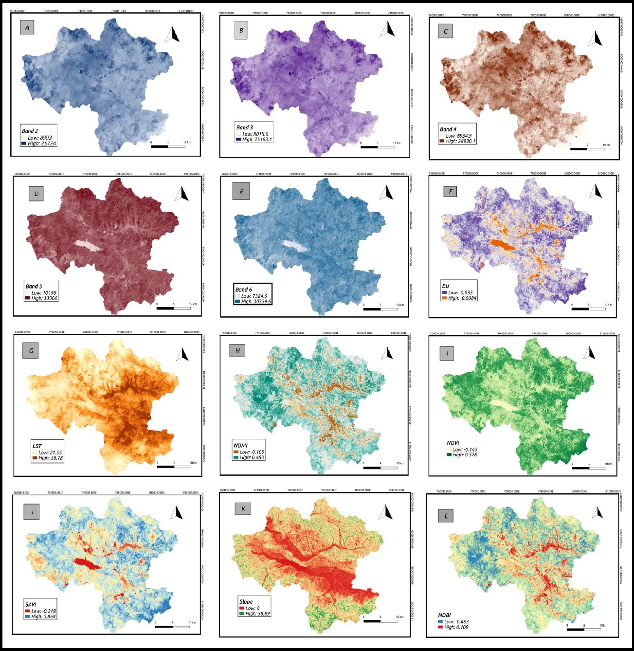
Although some researchers, such as Choubin et al. [17], maintain that no standard procedure exists for modelling PM, other researchers [18] have shown that meteorological parameters, terrain topography, roads and urban structure are factors that are significant in PM2.5 modelling studies. For our study, eleven (11) parameters were taken into account; these include Normalized Difference Vegetation Index (NDVI), Normalized Difference Moisture Index (NDMI), Land Surface Temperature (LST), slope, Soil-Adjusted Vegetation Index (SAVI), Band 2 (B2), Band 3 (B3), Band 4 (B4), Band 5 (B5), Band 6 (B6), and Built-up Index (BI). Landsat Operational Land Image (B2, B3, B4, B5 and B6) and Thermal Infrared Sensor (B10) bands were sourced from the landsat 8 collection catalogue. The surface indices LST, NDVI, NDMI, SAVI, Normalized Difference Built-up Index (NDBI) and BI ware derived from these bands. The bands and indices are shown in Figure 1. A slope map was also generated from the Shuttle Radar Topography Mission (SRTM) image using the spatial analysis tools in QGIS. All these bands and indices were queried with the GGE tool and further post-processed in QGIS Desktop 2.18.17.
Data aggregation, standardization and model preparation
QGIS 2.18.17, an open-source geospatial tool, was used to analyze the slope, ground truth data, including the buffer and grid, and satellite data. The buffer analysis was carried out using the vector processing tool in QGIS to create a 900 m radius around the monitoring stations, with the assumption that the PM2.5 concentration level remained the same within the established buffer zone. For the training dataset, a grid cell of 30 m x 30 m spatial resolution was created within the buffer zone. The data were exported to R studio 1.2.5001 in CSV format with 14514 points for further analysis. Data cleaning processes were carried out, and numerical values of PM2.5 were transformed into categorical variables for convenient machine learning model training.
All data sets were then standardized using the variance of a feature (Z), given as
xi = observation, μ = mean, and σ = standard deviation
The training and testing of the model were splitted by using 70% and 30% of the standardized data, respectively. Model training, hyperparameter optimization and evaluation were implemented with the aid of the CARET package within the R studio environment.
Air quality index
The air quality index (AQI) in table 1 is calculated based on the concentration levels of PM and gaseous pollutants, which can vary depending on the location and time of measurement. Public health risk increases as the AQI increases, especially in children, the aged, and vulnerable people. During these periods, the government encourages people to reduce outdoor activities or wear face masks to reduce risks. Different countries possess unique air quality indices that align with their respective national air quality regulations, which are the target class for predicting pollution levels. In Table 2 the PM2.5 values were used as the baseline to classify the concentration level estimated during the modelling.
Model evaluation and feature importance assessment
Machine learning algorithms, namely, XGBoost, K-Nearest Neighbor (KNN), and Naïve Bayes (NB), were utilized. These models were initially deployed with default parameters but were optimized via the grid method. Their performance was gauged using a suite of metrics, such as accuracy, precision, and Area Under the ROC Curve (AUC), among others. In particular, the AUC served as a valuable indicator of model accuracy. The model with the best performance was chosen to discern which variables were most crucial for predictions, with the importance of the features evaluated for each season. This feature assessment was conducted using the CARET package, employing the VarImp function. Consequently, the feature importance was evaluated using XGBoost to understand the significance of each feature in predicting PM2.5. By gauging the influence of different variables, deeper insights were obtained into the model's functioning.
Results
Exploratory analysis
The mean PM2.5 value for the three years across the four seasons was estimated as shown in Table 1, which serves as the target variables used in the models to predict PM2.5 pollution in Bosnia. The winter season had the highest PM2.5 concentration among the four seasons, while the summer season had the lowest concentration. BKC had a higher pollution concentration than other areas across all seasons except for summer. These insights were used in the ML models along with satellite and elevation data to predict ambient air pollution levels in the study area.
Model hyperparameters:
For XGBoost, the hyper-parameter with the highest model accuracy is as follows: n-rounds are 210 for winter and summer and 200 for autumn and spring; maximum tree depth for summer and winter is 6, while for spring and autumn, it is 18. The learning rate for summer differed from that of the other seasons. Moreso, for gamma, the summer and autumn seasons have the same values, and winter and spring have the same values. The min_child_weight and subsample use the same value for all four seasons. In the NB model, the laplace correction was 0.5 for the autumn season, while the other seasons used a value of 0. The bandwidth adjustment has the same value of 1 for spring and 0.5, for the winter, summer, and autumn seasons. For the KNN model, the number of nearest neighbors selected from the grid search was five for winter and three for the other seasons. The default distance metric used in the CARET library is the euclidean distance, and the k-value set at 3 exhibited the best accuracy among the other values.
Model performance evaluation
As displayed in Table 3, all models performed generally well. The results indicate that XGBoost consistently outperformed the other models in terms of all evaluation metrics. XGBoost demonstrated high sensitivity and kappa across all seasons, indicating its strong ability to correctly identify air quality cases with minimal misclassification. For example, in the winter season, XGBoost achieved the highest sensitivity and kappa. NB generally exhibited lower sensitivity than XGBoost and KNN in all seasons, with the lowest value occurring in the autumn season. However, the specificity of NB remained relatively high, particularly during the autumn season. Furthermore, KNN showed high sensitivity across all seasons, with the winter season having the highest value. Specificity was also consistently high for KNN throughout the seasons.
Across all seasons, XGBoost showed the highest AUC values, scoring the maximum possible value of 1 during winter. Implying that XGBoost is excellent in distinguishing between good and poor air quality. It also outperformed all other models' accuracy throughout all the seasons, with 0.85 in summer and 0.98 in winter. Even though NB and KNN models showed relatively good performance, the XGBoost model displayed superior performance, and thus, it is identified as the best model for expressing the air quality levels in this region.
Variable important assessment
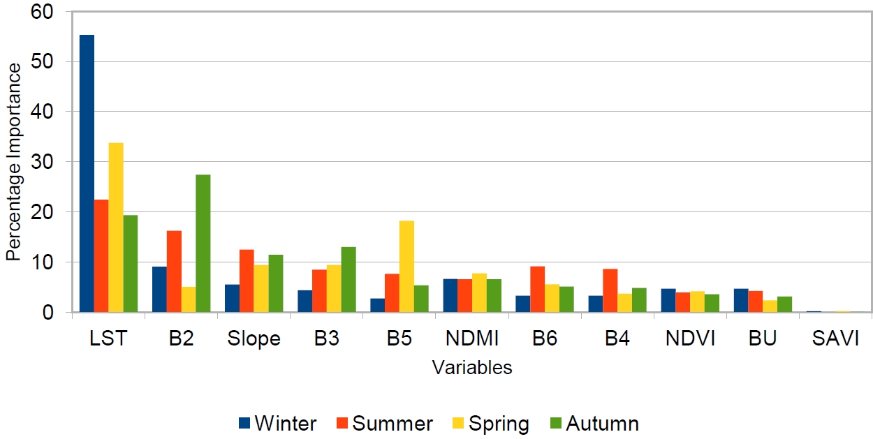
The XGBoost model performed the best, and was used to measure the most important variable influencing the PM2.5 concentration. Figure 3 gives details of level of significance of each variable in each season. Notably, all the variable showed some level of significance which varies with each season except for SAVI. All the selected variables have a varying level of correlation with the target variable. However, the XGB model identified that LST, B2, B3, B5, and slope significantly influenced the model during the various seasons. LST, a temperature index was identified as the most important air quality prediction variable for all seasons, with the highest contribution in the winter season. It is logical that LST can influence human activities and behaviors such as vehicular emissions, heating demands in cold weather etc., leading to amplified feedback to its surrounding environment. Moreover, the increased contribution of LST during the winter season can be attributed to reduced solar radiation, which leads to the formation of a stable atmospheric layer. This stability lowers the inversion capping towards the surface, trapping and elevating concentrations of PM2.5. Consequently, some other important variables may undergo significant changes that can affect their correlation with the air pollution level, thereby reducing their predictive power. On the other hand, SAVI exhibited the lowest importance with value less than 1 across the four seasons.
Generation of probability and classification map
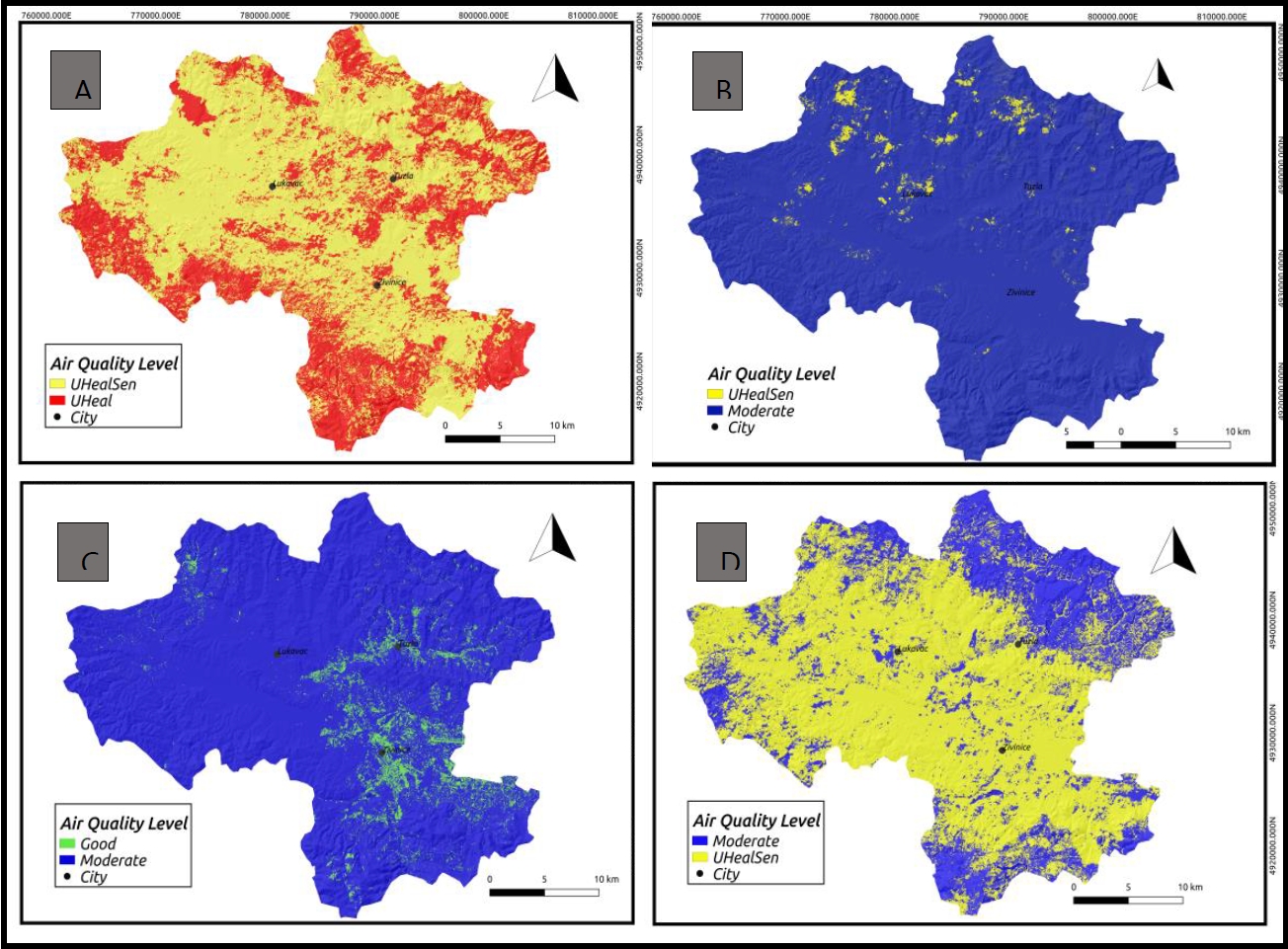
The probability map from the XGBoost, NB, and KNN models predicts that air quality during winter is unhealthy in some areas and capable of affecting sensitive individuals. In contrast, the summer season was predicted to have good and moderate air quality across all models. Regions close to the monitoring stations exhibited more extensive coverage of areas with good air quality during the summer across all models. Regions close to the monitoring stations exhibited more extensive coverage of areas with good air quality during the summer across all models. However, in the XGBoost model, there are some areas around the monitoring stations where the air quality (PM2.5 concentration) is uncertain, with the likelihood of being either good or moderate. In autumn and spring, air quality is predicted to be moderate and unhealthy for sensitive individuals. The output of the XGBoost model for the spring season differed from the air quality maps generated by the KNN and NB models. This is due to the higher percentage of the area being classified as having moderate air quality, at over 65 %, compared to the other two models.
The classification maps in Figure 2 were produced using the predicted output from the XGBoost model, which appeared to be more accurate than the other models. The probability maps for all seasons had the same air quality levels as the classification maps. The summer season, which has the best air quality (PM2.5 concentration) among all the models, is healthy for all inhabitants, including sensitive and vulnerable individuals. In contrast, the winter season has the worst air quality, which is unhealthy for all inhabitants, particularly those living around areas at the extreme end of the study area in Tuzla Canton, posing a significant concern.
Discussion
The use of machine learning models for modelling air quality levels, particularly for particulate matter (PM2.5 and PM10) and other pollutants, can be an effective solution in areas with limited in-situ air quality measurement data where conventional spatial interpolation methods cannot be applied because of a lack of data. This was demonstrated in the present study, as previously described by Wang et al. [20]. Usually, many predictors, such as road density [18,21,22], MODIS AOD [13,23,24], meteorological data [12,13,23,24], Landsat 8 bands and Indices [12,18,21], and topography [25], are applied to predicting the PM2.5 air quality level. However, in this study, we used only Landsat 8 bands, environmental indices, and slope to estimate the PM2.5 air quality. The model identifies the important variables for each season based on the correlation between those variables and PM2.5 concentration. Through this approach, the model established that the variables LST, B2, B3, B5, and SLOPE had a good correlation in predicting the PM2.5 concentrations across most seasons.
Meanwhile, afforestation trends in BiH indicate that the afforestation volume decreased [26], which could explain why SAVI does not have a significant influence on predicting air quality in Tuzla, as the vegetation might be sparse and the soil in most areas is bright. The reflectance of the soil might have a greater impact, potentially resulting in low SAVI values, thereby affecting its usefulness in predicting air pollution. In contrast, B2 was determined to be the most significant variable among the selected bands, especially in summer and autumn. This may indicate that more vegetation was present during these seasons, which can lead to better air quality. This is supported by the fact that NDVI and NDMI, which are other indices commonly used to estimate vegetation health, also had slightly fair values in these seasons. Across all seasons, LST was the most important variable in predicting the PM2.5 air quality level. In Europe, Bosnia is among the countries with the highest temperature; this impact cannot be overemphasized in air pollutant emissions. Considering that higher temperatures affect the movement of air pollution and can accelerate chemical reactions, leading to increased volatilization of pollutants, there could be a spike in the concentration of PM2.5 [27].
The air quality level of a specific region can vary depending on the emission source and geographical location [28]. The use of some of these variables could also influence the effectiveness of the air pollution model. Anthropogenic activities and the impact of traffic in densely populated areas could increase PM2.5. The use of traffic emissions from vehicular activities performed the best among the variables in predicting particulate using the ANN model [29]. In Bosnia, there have been several records of wildfires during many periods, especially in the summer, due to climate change [30], which the high topography factor could influence [31]. During wildfire events, the emission of toxic gases can influence the increase in particulate matter; this could be the main reason why the slope is highly important in the prediction of PM2.5 concentration in the summer season. Although MODIS AOD products have good applicability in estimating particulate matter [27], their shortcomings cannot be ignored as using products that have a spatial resolution, such as (6 km by 6 km or 10 km by 10 km) in small and medium study areas, such as the one used in this case study, may not be practicable because some features may not be well represented. In some previous studies, the use of MODIS products in some study areas did not perform relatively well in terms of quality [32] and in comparison with landsat 8 products [12].
The best model was selected as the XGBoost model, following the assessment of the metrics. Notably, the best model depends on a specific problem and the desired trade-off between sensitivity and specificity. According to the results presented in Figure 3, it was observed that an increase in PM2.5, air quality level was experienced in the winter season and at its highest concentration around the extreme end of the study area, which are highlands and peaks and within the urbanized area in the Tuzla canton, and also the best air quality was recorded in the summer. Moreover, the model‘s classification map is reliable when compared with the real-time live AQI index (available at https://www.iqair.com/air-quality-map), underscoring its potential for practical air quality monitoring and its credibility for future air quality prediction.
The dynamics of the atmospheric boundary layer largely influence the seasonal fluctuation. In winter, air parcels containing pollutants, such as PM, become cooler than the surrounding atmosphere. This creates negative buoyancy, causing these polluted air parcels to be trapped near the ground due to temperature inversions. Conversely, in summer, warmer air parcels rise due to surface heating, which induces convection in the surface layer. This process enhances turbulence and mixing effectively, aiding the dispersion and diminishing their concentration. The elevated pollution levels during the winter, particularly in the highlands, can also be attributed to additional pollution sources, such as fossil fuel burning for heating and cooking, along with emissions from outdated vehicles. Emissions from these sources can accumulate in valleys or basins because of the influence of terrain on air circulation [33]. Hence, stringent regulations should be implemented to control and manage these increased PM2.5 air quality levels in the winter to bring the unhealthy air quality to an acceptable level.
Conclusions
This study aimed to develop machine learning classification models to predict the likelihood of PM2.5 in Tuzla Canton, BiH. For this purpose, we investigated how landsat 8 bands and environmental indices can contribute to predicting PM2.5 concentration. The performance of the models in evaluating the effect of the PM2.5 air quality level in different seasons was also compared. The XGBoost model and KNN performed better than the NB model in predicting PM2.5 air quality concentrations. For the XGBoost model, LST, B2, and slope were the most contributing variables in predicting the concentration of PM2.5, across the four seasons. This is the first study to investigate the importance of using landsat 8 bands and their corresponding derived indices and topography for PM2.5 air quality concentration prediction in the BiH. A reasonable performance was achieved in predicting the air quality level across all four seasons.
While the use of meteorological parameters such as wind speed and direction, precipitation, traffic factors, and industrial emission data has been important predictors for predicting PM2.5 air quality concentrations, we recommend incorporating these features with landsat 8 bands and indices to improve the prediction of PM2.5 air quality levels more accurately, particularly in seasons with less performance. It is important to conduct feature importance assessments to optimally select variables and address overfitting or underfitting issues before mapping air quality. These issues apply to all machine learning models to varying degrees. We acknowledge that some bias arose in our data selection which might result in the underfitting of our model, some of which could owe to data availability issues as the monitoring stations used at the time of data collection were unevenly distributed.
It is also worth noting to compare the results obtained from landsat 8 products with MODIS AOD products, which have also proven useful in predicting particulate matter in some other studies. This insightful information can assist government decision-making in areas where it is crucial to prioritize the implementation of air quality regulations.